Making System Stacking Fingerprints (SSFs)#
This pipeline creates System Stacking Fingerprints (SSFs) like the one below which can be used to analyze system-wide pi-stacking in a molecular dynamics trajectory.
Load Trajectory#
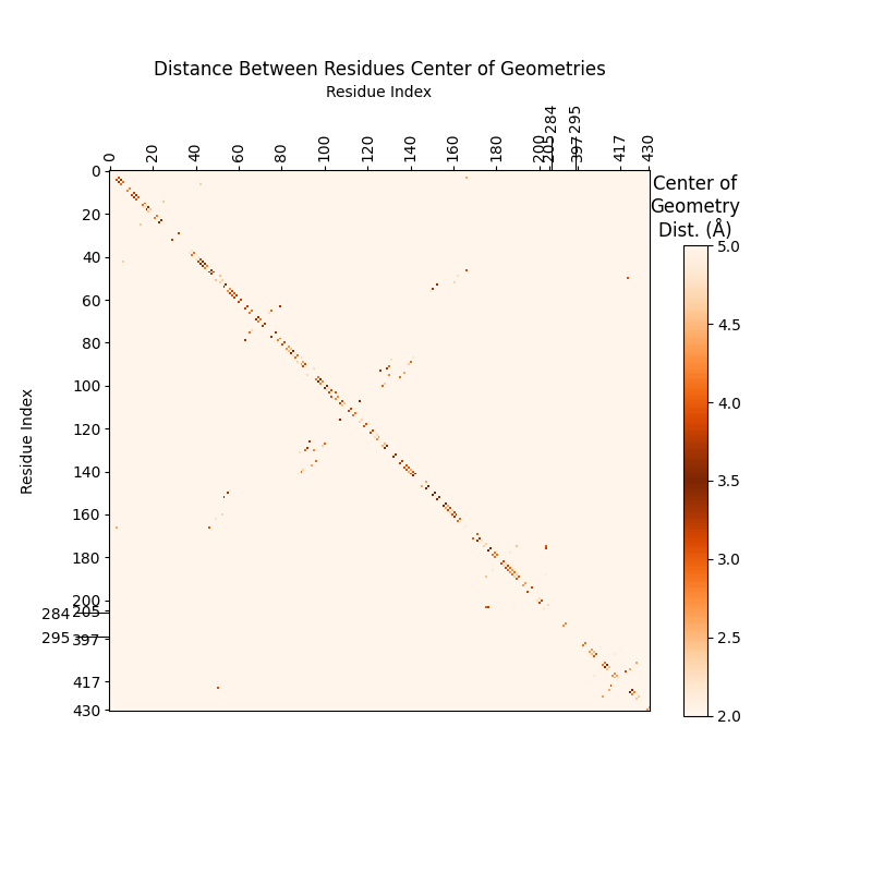
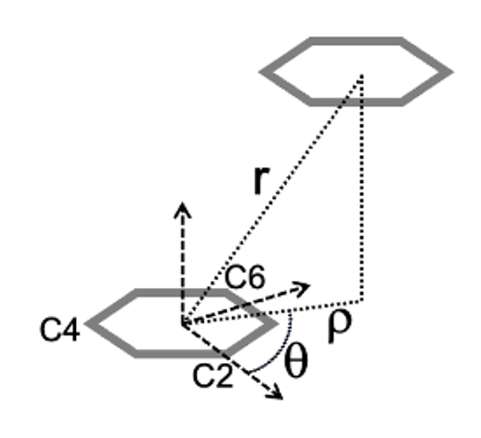
To analyze pi-stacking between two nucleotides, we compare their center of
geometry (COG) distance, the distance between the centers of their 6-membered
(pyrimidine) rings (see r below). For this, the only atoms we need are C2, C4, and C6 to triangulate
the COG of each ring.
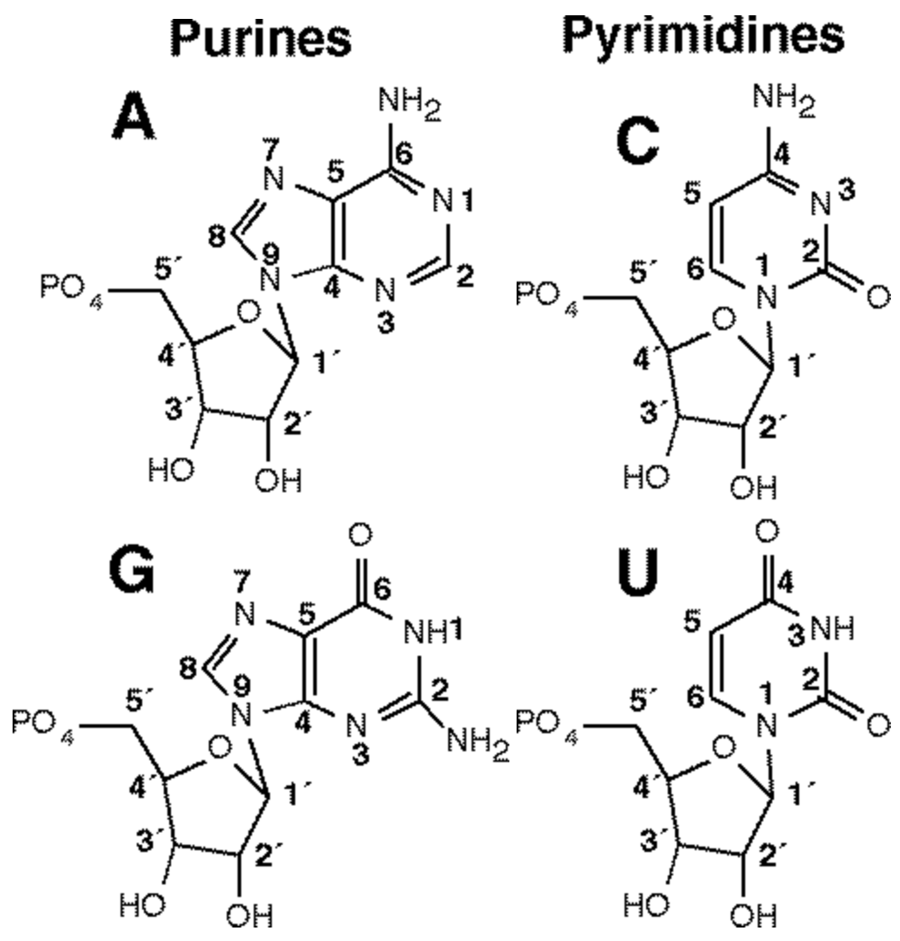
For reference, the Carbon Numbering of each nucleotide:
In this example pipeline, we use a trajectory of the Ribosome CAR-mRNA Interaction Surface found in the StACKER GitHub Repository. We filter this trajectory to the pi-stacking residue pair.
MD Files are provided for testing convenience in the testing folder:
first10_5JUP_N2_tUAG_aCUA_+1GCU_nowat.mdcrd: A 10-frame trajectory file with all atoms/residues.5JUP_N2_tUAG_aCUA_+1GCU_nowat.prmtop: The associated Topology File with the above trajectory.
We filter to atoms C2, C4, and C6 using filter_traj():
>>> import stacker as st
>>> filtered_traj = st.filter_traj("first10_5JUP_N2_tUAG_aCUA_+1GCU_nowat.mdcrd",
...                 top_file = "5JUP_N2_tUAG_aCUA_+1GCU_nowat.prmtop",
...                 atoms = {"C2", "C4", "C6"})
WARNING: Residue Indices are expected to be 1-indexed
Reading trajectory...
Reading topology...
Filtering trajectory...
WARNING: Output filtered traj atom, residue, and chain indices are zero-indexed
>>> filtered_traj
<mdtraj.Trajectory with 10 frames, 756 atoms, 252 residues, without unitcells at 0x1164eab10>
Now the Python variable filtered_traj contains 10 frames of C2, C4, C6 information for all nucleotides.
Calculate Distance Between Residues#
Immediately, we can check if a residue pair is pi-stacking in a given frame. We calculate
the distance between the COG of two residues using calculate_residue_distance().
COG distance close to 3.5 Å indicates pi-stacking. For instance, the A-site mRNA codons
(residues 422, 423, and 424) are likely pi-stacking:
>>> distance_vec = st.calculate_residue_distance(
...     filtered_traj,
...     res1 = 422,
...     res2 = 423,
...     frame = 3
... )
>>> distance_vec.magnitude()
3.509042
Create a System Stacking Fingerprint (SSF)#
An SSF calculates the COG distance for all nucleotide pairs in a trajectory frame.
The result is a square matrix where position (i, j) represents the distance
from residue i to residue j. This is done with get_residue_distance_for_frame()
The filtered_traj object has 252 residues, so we create a 252 x 252 SSF:
>>> ssf = st.get_residue_distance_for_frame(filtered_traj, frame = 2, write_output = True)
Loading: [####################################################################################################] Current Residue: 252/252 (100.0%)
Frame 2 done.
>>> ssf.shape
(252, 252)
We can calculate the SSF for multiple frames of a trajectory using system_stacking_fingerprints(), which
accepts smart indexing of frames (eg. 1-3,15-17 = 1,2,3,15,16,17):
>>> ssfs = st.system_stacking_fingerprints(filtered_traj, frames = '1-3')
>>> ssfs.shape
(3, 252, 252)
ssfs is now a list, where ssfs[i] is the SSF for frame i (0-indexed frame). If frames is empty,
the SSF will be calculated for all frames. For multi-frame
trajectories, it is recommended to use the threads option to parallelize, calculating the SSF for multiple
frames at once. When parralelizing, turn off standard output with write_output:
>>> ssfs = st.system_stacking_fingerprints(
...     filtered_traj,
...     frames = '1-10',
...     threads = 10,
...     write_output = False
... )
>>> ssfs.shape
(10, 252, 252)
Get the Average SSF for a Trajectory#
Single-frame SSFs are rarely as illuminating as the average SSF for all frames
of a trajectory. Users can create this using get_frame_average(), using the
output from system_stacking_fingerprints() in the step above:
>>> ssfs = st.system_stacking_fingerprints(
...     filtered_traj,
...     frames = '1-10',
...     threads = 10,
...     write_output = False
... )
>>> avg_ssf = st.get_frame_average(ssfs)
>>> avg_ssf.shape
(252, 252)
avg_ssf contains averaged stacking information throughout the trajectory.
The next step shows how to analyze these results.
How to Visualize an SSF#
display_ssfs() will visualize SSFs in Python output, with each SSF frame
as a frame of the video:
>>> import stacker as st
>>> filtered_traj = st.filter_traj("first10_5JUP_N2_tUAG_aCUA_+1GCU_nowat.mdcrd",
...                 top_file = "5JUP_N2_tUAG_aCUA_+1GCU_nowat.prmtop",
...                 atoms = {"C2", "C4", "C6"})
WARNING: Residue Indices are expected to be 1-indexed
Reading trajectory...
Reading topology...
Filtering trajectory...
WARNING: Output filtered traj atom, residue, and chain indices are zero-indexed
>>> ssfs = st.system_stacking_fingerprints(
...     filtered_traj,
...     frames = '1-10',
...     threads = 10,
...     write_output = False
... )
>>> resSeqs = [res.resSeq for res in filtered_traj.topology.residues]
>>> st.display_ssfs(
...     ssfs,
...     res_indicies = resSeqs,
...     seconds_per_frame = 2
... )
It is recommended to run get_frame_average() and then save the output
as a .png for comparison with other trajectories:
>>> import stacker as st
>>> filtered_traj = st.filter_traj("first10_5JUP_N2_tUAG_aCUA_+1GCU_nowat.mdcrd",
...                 top_file = "5JUP_N2_tUAG_aCUA_+1GCU_nowat.prmtop",
...                 atoms = {"C2", "C4", "C6"})
WARNING: Residue Indices are expected to be 1-indexed
Reading trajectory...
Reading topology...
Filtering trajectory...
WARNING: Output filtered traj atom, residue, and chain indices are zero-indexed
>>> ssfs = st.system_stacking_fingerprints(
...     filtered_traj,
...     frames = '1-10',
...     threads = 10,
...     write_output = False
... )
>>> avg_ssf = st.get_frame_average(ssfs)
>>> ssfs = [avg_ssf]
>>> resSeqs = [res.resSeq for res in filtered_traj.topology.residues]
>>> st.display_ssfs(
...     ssfs,
...     resSeqs,
...     tick_distance = 20,
...     outfile = "SSF_test.png",
...     scale_limits = (2,5),
...     xy_line = False
... )
Command Line Options offers many future analyses,
including combining SSF images along the x=y line for visual comparison
with stacker -s ssf -B and stacker -s compare.
How to Analyze an SSF#
get_top_stacking() will give the stacking pairs with the most
pi-stacking (ie. closest to 3.5Å):
>>> st.get_top_stacking(
...     filtered_traj,
...     avg_ssf
...     )
Res1    Res2    Avg_Dist
117     108     3.43
153     54      3.35
56      151     3.34
94      127     3.67
93      130     3.68
It is recommended to save the output to a .csv and use the other parameters
for get_top_stacking() to prepare for future analyses using the
Command Line Options:
>>> st.get_top_stacking(
...     filtered_traj,
...     avg_ssf,
...     csv = 'top_stacking.csv',
...     n_events = -1,
...     include_adjacent = True
... )
In the command line, [user]$ stacker -s compare can give the residue
pairs that changed the most between trajectories, by inputting two csv
outputs from get_top_stacking(). Use [user]$ stacker -s compare --help
for more information.
Using K Means#
You can compare multiple System Stacking Fingerprints via K-Means. The algorithm takes multiple SSFs with no knowledge of their trajectory and groups similar SSFs. Thus, the algorithm groups trajectories via similar system-wide stacking.
Note: the SSFs must be comparable, meaning an equal amount of residues.
With StACKER’s Command Line Options, the .txt
files below were created:
testing/5JUP_N2_tGGG_aCCU_+1GCU_data.txt.gz: numpy array with 3200 SSFstesting/5JUP_N2_tGGG_aCCU_+1GCU_data.txt.gz: numpy array with 3200 SSFs
These files are too large to provide, but can be made with stacker -s ssf -d.
They can be read as Python objects and reshaped:
>>> import numpy as np
>>> import math
>>> GCU_3200_flattened_ssfs = np.loadtxt('../testing/5JUP_N2_tGGG_aCCU_+1GCU_data.txt.gz')
>>> GCU_3200_flattened_ssfs.shape
(3200, 16129)
>>> GCU_3200_ssfs = GCU_3200_flattened_ssfs.reshape(GCU_3200_flattened_ssfs.shape[0], math.isqrt(GCU_3200_flattened_ssfs.shape[1]), math.isqrt(GCU_3200_flattened_ssfs.shape[1]))
>>> GCU_3200_ssfs.shape
(3200, 127, 127)
- Or the files can be read and prepared for KMeans data
with
read_and_preprocess_data()andrun_kmeans():>>> import stacker as st >>> data_arrays = st.read_and_preprocess_data( ... ["testing/5JUP_N2_tGGG_aCCU_+1CGU_data.txt.gz", ... "testing/5JUP_N2_tGGG_aCCU_+1GCU_data.txt.gz"] ... ) >>> st.run_kmeans(data_arrays, n_clusters = 2) (6400, 16129) For n_clusters = 2 The average silhouette_score is : 0.10815289849518733 Dataset: 5JUP_N2_tGGG_aCCU_+1CGU_data Cluster 1: 0 matrices Cluster 2: 3200 matrices Dataset: 5JUP_N2_tGGG_aCCU_+1GCU_data Cluster 1: 3120 matrices Cluster 2: 80 matrices
So the SSFs from the two datasets are distinct enough to separate into two clusters.
We can visualize this with plot_cluster_trj_data():
>>> import stacker as st
>>> data_arrays = st.read_and_preprocess_data(
... ["testing/5JUP_N2_tGGG_aCCU_+1CGU_data.txt.gz",
... "testing/5JUP_N2_tGGG_aCCU_+1GCU_data.txt.gz"]
... )
>>> st.run_kmeans(data_arrays, n_clusters = 7, outdir = 'testing/')
(6400, 16129)
For n_clusters = 7 The average silhouette_score is : 0.09968523895626617
Dataset: 5JUP_N2_tGGG_aCCU_+1CGU_data
Cluster 1: 560 matrices
Cluster 2: 0 matrices
Cluster 3: 240 matrices
Cluster 4: 0 matrices
Cluster 5: 1138 matrices
Cluster 6: 2 matrices
Cluster 7: 1260 matrices
Dataset: 5JUP_N2_tGGG_aCCU_+1GCU_data
Cluster 1: 80 matrices
Cluster 2: 1057 matrices
Cluster 3: 0 matrices
Cluster 4: 738 matrices
Cluster 5: 0 matrices
Cluster 6: 1245 matrices
Cluster 7: 80 matrices
Results written to: testing/clustering_results_7.txt
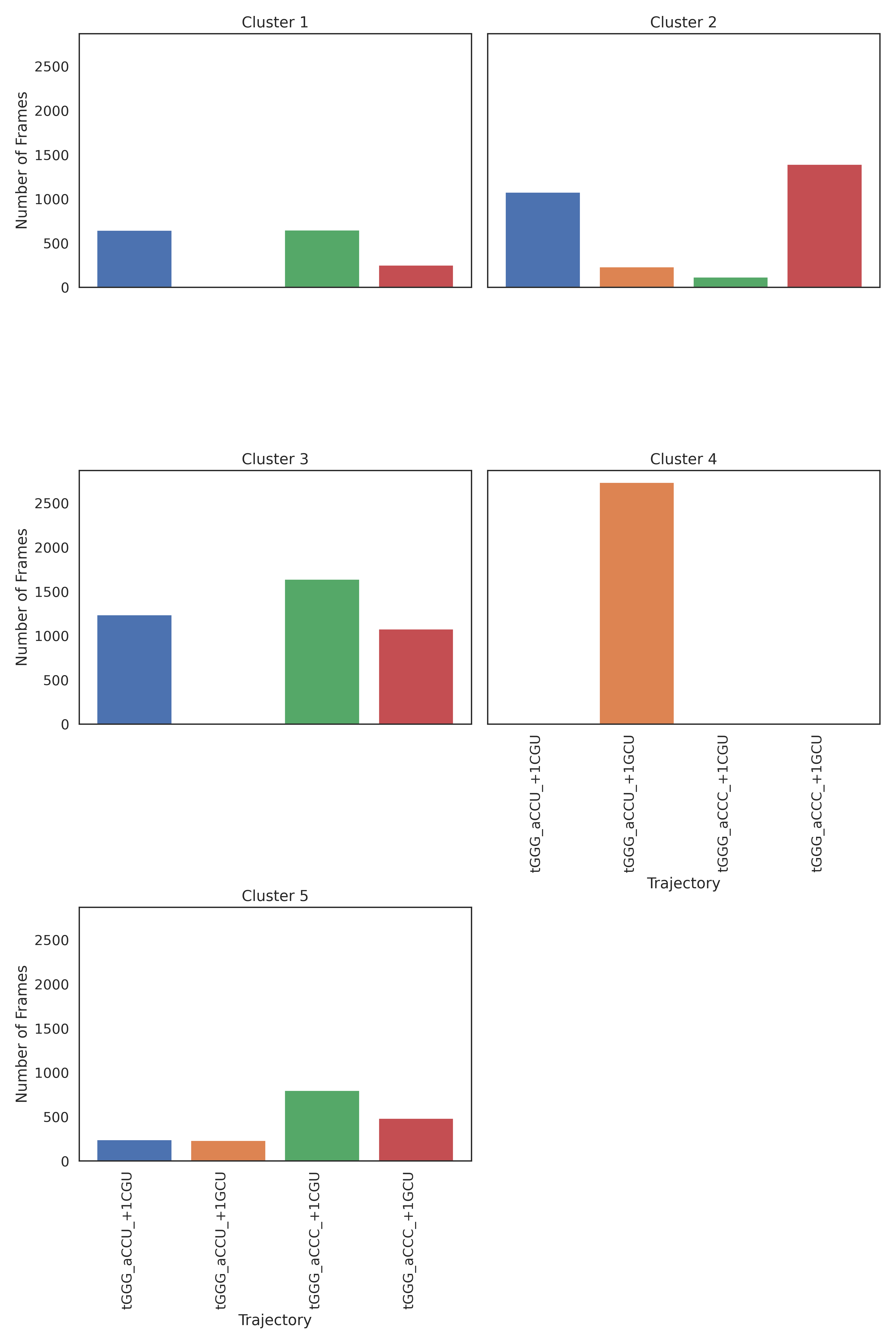
>>> st.plot_cluster_trj_data("testing/clustering_results_7.txt", "testing/kmeans_plot.png", {'5JUP_N2_tGGG_aCCU_+1CGU_data': 'tGGG_aCCU_+1CGU', '5JUP_N2_tGGG_aCCU_+1GCU_data': 'tGGG_aCCU_+1GCU'})
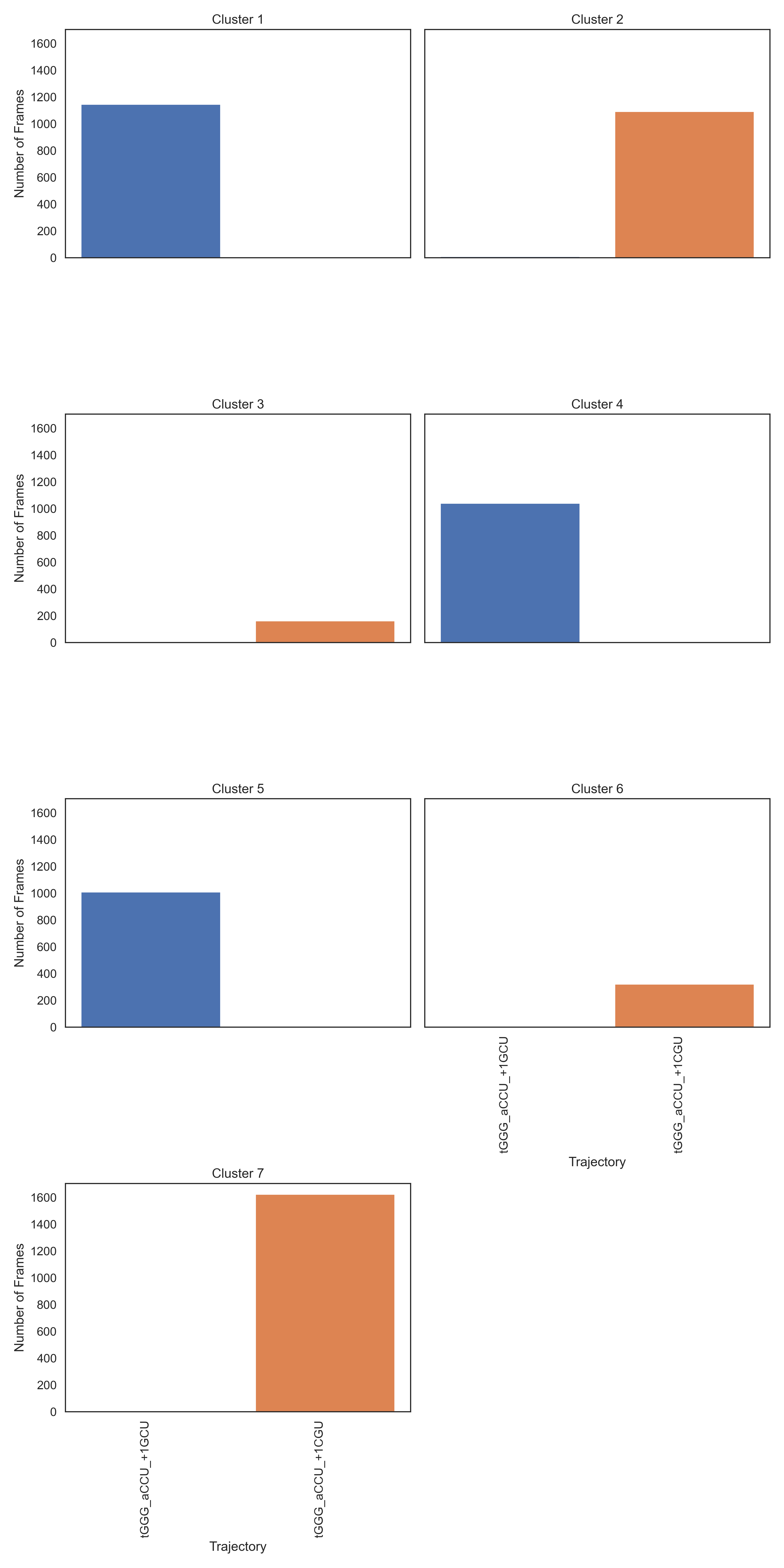
The SSFs still split into distinct clusters (there is no cluster with a significant contribution from both trajectories), meaning the structures have different pi-stacking.
Picking the Right Number of Clusters#
StACKER is equipped to run Silhouette Analysis
in order to select the correct number of clusters. plot_silhouette()
can create Silhouette Plots:
>>> import stacker as st
>>> data_arrays  = st.read_and_preprocess_data(
...     ["testing/5JUP_N2_tGGG_aCCU_+1CGU_data.txt.gz",
...     "testing/5JUP_N2_tGGG_aCCU_+1GCU_data.txt.gz"]
... )
Reading data: 5JUP_N2_tGGG_aCCU_+1CGU_data.txt.gz
Reading data: 5JUP_N2_tGGG_aCCU_+1GCU_data.txt.gz
>>> blinded_data = st.create_kmeans_input(data_arrays)
(6400, 16129)
>>> for n_cluster in range(2,8):
...     st.run_kmeans(data_arrays, n_clusters = n_cluster, outdir = 'testing/')
...     st.plot_silhouette(n_cluster, blinded_data, outdir = 'testing/')
(6400, 16129)
For n_clusters = 2 The average silhouette_score is : 0.10815289849518733
Dataset: 5JUP_N2_tGGG_aCCU_+1CGU_data
        Cluster 1: 0 matrices
        Cluster 2: 3200 matrices
Dataset: 5JUP_N2_tGGG_aCCU_+1GCU_data
        Cluster 1: 3120 matrices
        Cluster 2: 80 matrices
Results written to: ../testing/clustering_results_2.txt
File saved to: ../testing/silhouette2.png
(6400, 16129)
For n_clusters = 3 The average silhouette_score is : 0.11018525011212786
Dataset: 5JUP_N2_tGGG_aCCU_+1CGU_data
        Cluster 1: 720 matrices
        Cluster 2: 0 matrices
        Cluster 3: 2480 matrices
Dataset: 5JUP_N2_tGGG_aCCU_+1GCU_data
        Cluster 1: 0 matrices
        Cluster 2: 3194 matrices
        Cluster 3: 6 matrices
Results written to: ../testing/clustering_results_3.txt
File saved to: ../testing/silhouette3.png
...
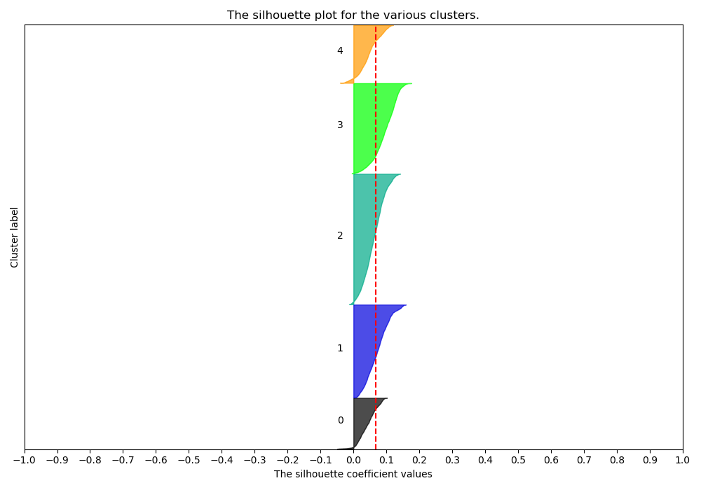
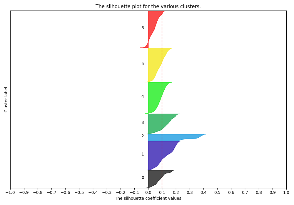
Silhouette Plots show the distance of all points in a cluster from the cluster’s centroid. We want plots with clusters of similar size along the y-axis and with most points around the same distance from 0 on the x-axis. A Cluster choice of 6 is appropriate:
testing/silhouette6.png
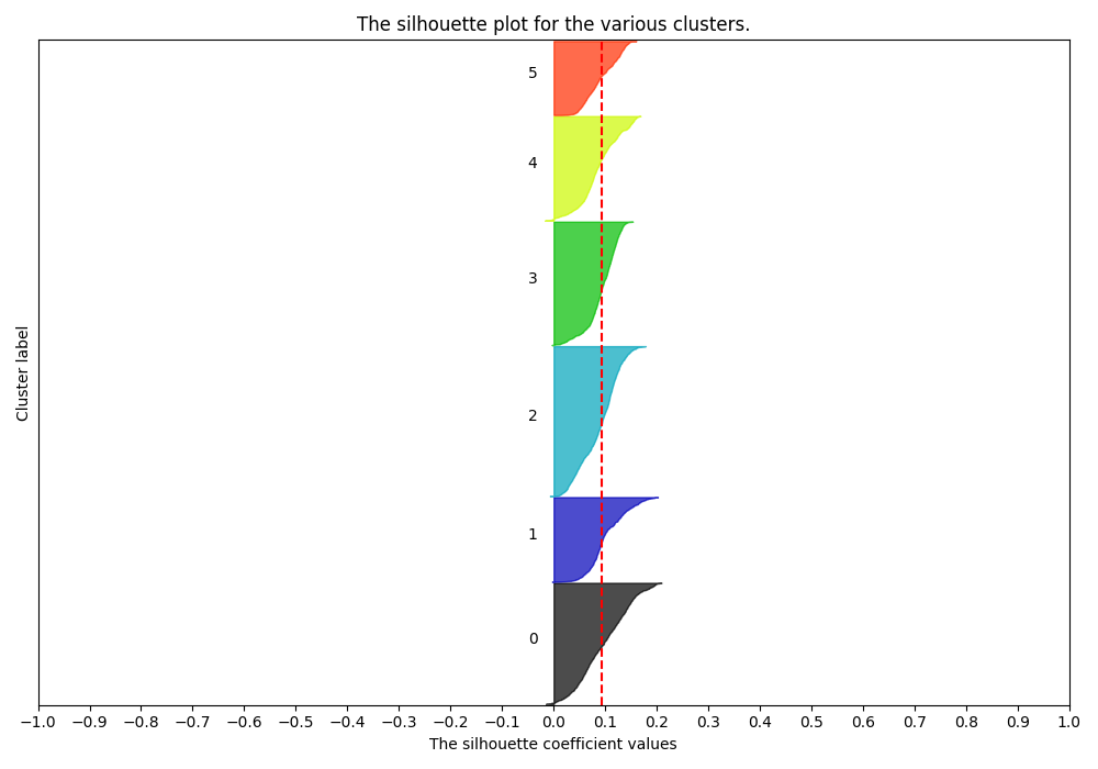
While a cluster choice of 7 is not:
testing/silhouette7.png
Principal Component Analysis#
KMeans on SSF gathers Euclidean Distance on multi-dimensional vectors that are impossible to plot. We can, however, do a heuristic plotting of these SSFs using Principal Component Analysis (PCA).
First, we can plot the un-blinded SSFs and color them by their trajectory of origin.
We have 3200 frames worth of SSFs for each trajectory, and we plot them using
plot_pca():
>>> import stacker as st
>>> dataset_names = ["testing/5JUP_N2_tGGG_aCCU_+1CGU_data.txt.gz",
...     "testing/5JUP_N2_tGGG_aCCU_+1GCU_data.txt.gz"]
>>> data_arrays  = st.read_and_preprocess_data(
...     dataset_names
... )
Reading data: 5JUP_N2_tGGG_aCCU_+1CGU_data.txt.gz
Reading data: 5JUP_N2_tGGG_aCCU_+1GCU_data.txt.gz
>>> blinded_data = st.create_kmeans_input(data_arrays)
(6400, 16129)
>>> st.plot_pca(blinded_data, dataset_names, 'dataset')
This creates a PCA plot where each point is a frame of a trajectory,
plotted using the information solely from the SSF. The points are colored
by the trajectory dataset of origin. This outputs to a .png:
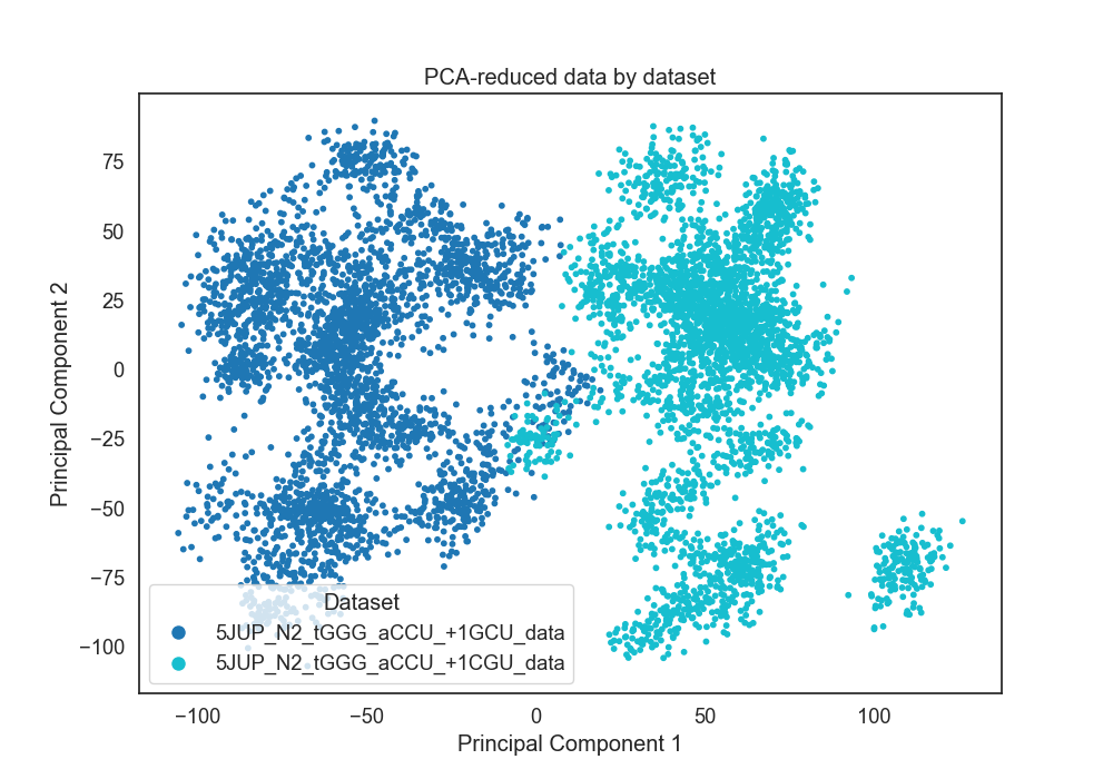
Here the SSFs from the two datasets separate cleanly, indicating
significantly different system-wide stacking. The PCA Plots can
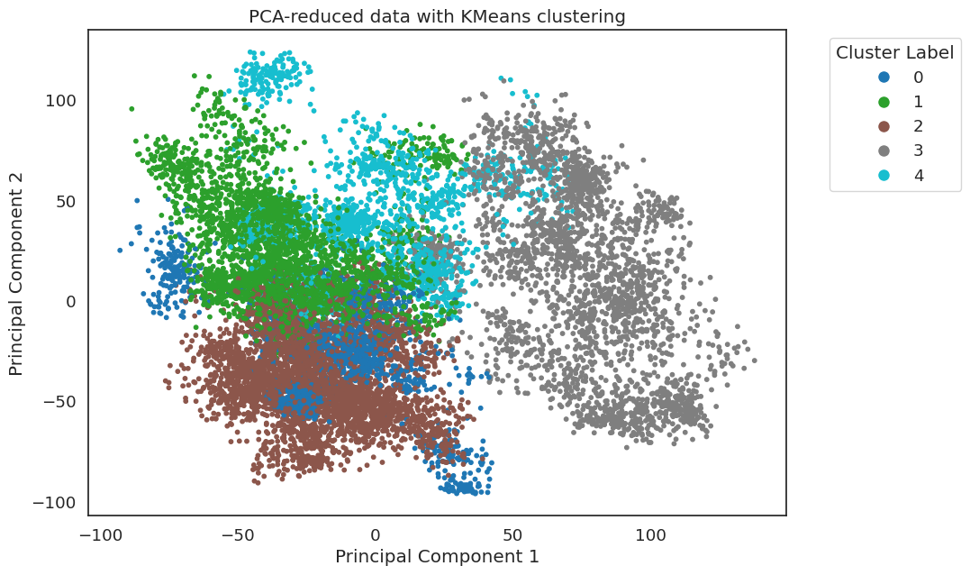
also be colored by kmeans result. Here, the frames are colored by
their KMeans result with 6 clusters:
>>> import stacker as st
>>> data_arrays  = st.read_and_preprocess_data(
...     ["testing/5JUP_N2_tGGG_aCCU_+1CGU_data.txt.gz",
...     "testing/5JUP_N2_tGGG_aCCU_+1GCU_data.txt.gz"]
...     )
Reading data: 5JUP_N2_tGGG_aCCU_+1CGU_data.txt.gz
Reading data: 5JUP_N2_tGGG_aCCU_+1GCU_data.txt.gz
>>> blinded_data = st.create_kmeans_input(data_arrays)
(6400, 16129)
>>> kmeans_results = st.run_kmeans(data_arrays, n_clusters=6)
(6400, 16129)
For n_clusters = 6 The average silhouette_score is : 0.09343055568735036
Dataset: 5JUP_N2_tGGG_aCCU_+1CGU_data
        Cluster 1: 0 matrices
        Cluster 2: 0 matrices
        Cluster 3: 1459 matrices
        Cluster 4: 4 matrices
        Cluster 5: 1017 matrices
        Cluster 6: 720 matrices
Dataset: 5JUP_N2_tGGG_aCCU_+1GCU_data
        Cluster 1: 1179 matrices
        Cluster 2: 824 matrices
        Cluster 3: 0 matrices
        Cluster 4: 1197 matrices
        Cluster 5: 0 matrices
        Cluster 6: 0 matrices
>>> st.plot_pca(blinded_data, dataset_names, coloring = 'kmeans', cluster_labels=kmeans_results)
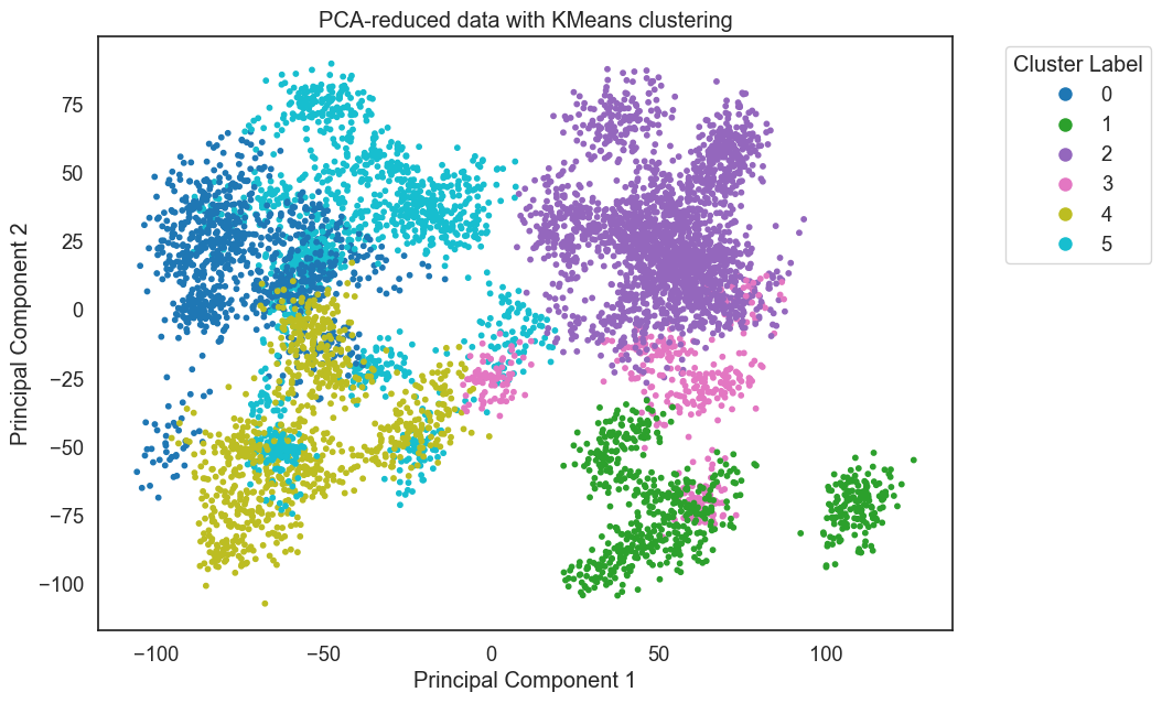
Each trajectory has three clusters, with no cluster capturing significant frames from both trajectories.
Finally, they can be colored by dataset but use facet to show each
dataset’s points on a separate PCA Grid. This helps with viewing multiple
datasets:
>>> import stacker as st
>>> dataset_names = ["/home66/esakkas/STACKER/DATA/5JUP_N2_tGGG_aCCU_+1CGU_data.txt.gz",
...     "/home66/esakkas/STACKER/DATA/5JUP_N2_tGGG_aCCU_+1GCU_data.txt.gz",
...     "/home66/esakkas/STACKER/DATA/5JUP_N2_tGGG_aCCC_+1CGU_data.txt.gz",
...     "/home66/esakkas/STACKER/DATA/5JUP_N2_tGGG_aCCC_+1GCU_data.txt.gz"
...     ]
>>> data_arrays = st.read_and_preprocess_data(dataset_names)
>>> blinded_data = st.create_kmeans_input(data_arrays)
(12800, 16129)
>>> st.plot_pca(blinded_data, dataset_names, 'facet')
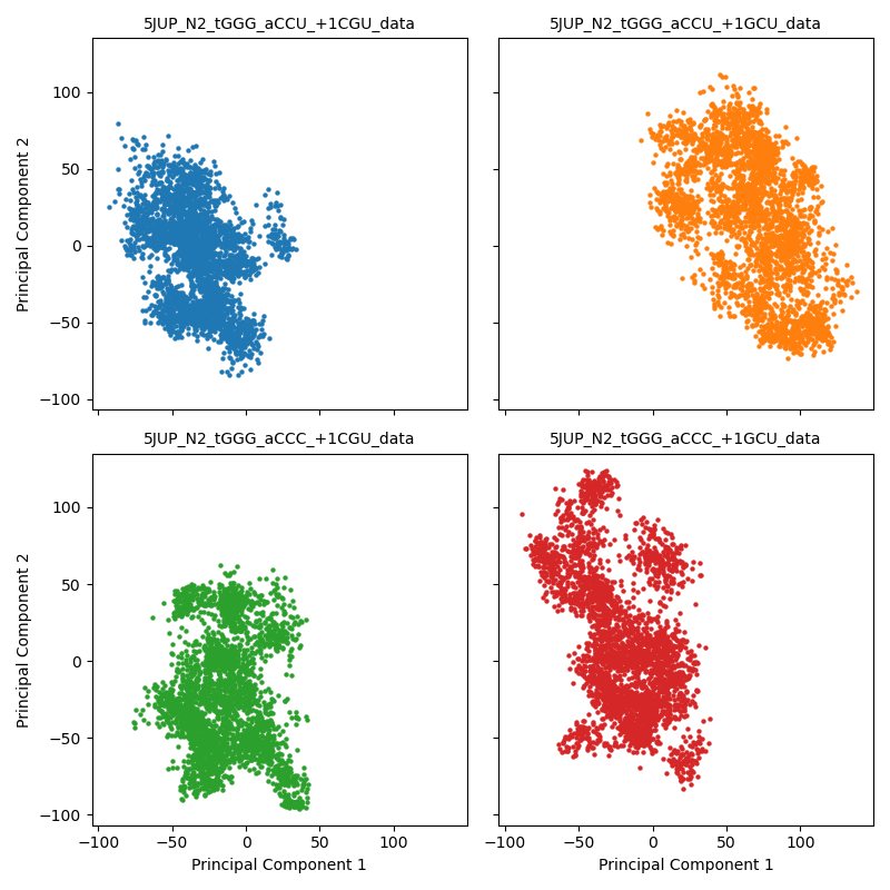
Here we see that the tGGG_aCCU_+1GCU trajectory occupies its own space.
We can combine this result with the KMeans and PCA plots below to strongly support
the conclusion that tGGG_aCCU_+1GCU has a different system-wide stacking,
and therefore a different structure, than the other three trajectories. The
K-Means results with the best silhouette plot is shown here: